Comparison with other models • lnmixsurv

This vignette shows a brief comparison of the survival_ln_mixture with other survival models, available through censored.

We begin by loading the packages and preparing the data.

library(lnmixsurv)
library(readr)
require(censored)
require(purrr)
require(dplyr)
require(ggplot2)

set.seed(4)

# Gerando dados
data <- simulate_data(n = 6000, k = 3, mixture_components = 2, 
                      percentage_censored = 0.3)$data |> 
  filter(t < 500) |> 
  rename(x = cat, y = t) 

new_data <- data |>
  distinct(x)

formula <- Surv(y, delta) ~ x

For comparison, lets also estimate the Kaplan-Meier survival function.

library(ggsurvfit)

km <- survfit2(formula, data)

surv_km <- tidy_survfit(km, type = "surv") |>
  select(.eval_time = time, .pred_survival = estimate, id = strata) |>
  tidyr::nest(.pred = c(.eval_time, .pred_survival))

The we build our parsnip specifications and store them in a list.

ln_survival <- survival_reg(dist = "lognormal") |>
  set_engine("survival")

ph_survival <- proportional_hazards() |>
  set_engine("survival")

decision_tree <- decision_tree(cost_complexity = 0) |>
  set_engine("rpart") |>
  set_mode("censored regression")

ln_mixture <- survival_reg() |>
  set_engine("survival_ln_mixture",
             iter = 4000, warmup = 2000, starting_seed = 10, 
             em_iter = 450, mixture_components = 3)

ln_mixture_em <- survival_reg() |>
  set_engine("survival_ln_mixture_em",
             iter = 250, starting_seed = 15, 
             mixture_components = 3)

specs <- list(
  ln_survival = ln_survival, ph_survival = ph_survival, ln_mixture = ln_mixture, decision_tree = decision_tree, ln_mixture_em = ln_mixture_em
)

Finally, thanks to the great parsnip API, we can fit and predict all models at once.

set.seed(1)

models <- map(specs, ~ fit(.x, formula, data))

pred_sob <- map(models, ~ predict(.x, new_data,
                                  type = "survival",
                                  eval_time = seq(500)))

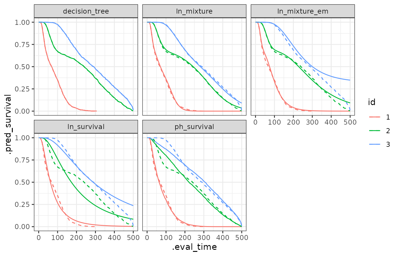
The following plot compares each model with the Kaplan-Meier estimates of the survival function.

all_preds <- bind_rows(pred_sob, .id = "modelo") |>
  group_by(modelo) |>
  dplyr::mutate(id = new_data$x) |>
  ungroup() |>
  tidyr::unnest(cols = .pred)

km_fit <- surv_km |>
  tidyr::unnest(cols = .pred) |>
  filter(.eval_time < 500)

ggplot(aes(x = .eval_time, y = .pred_survival, col = id), data = all_preds) +
  theme_bw() +
  geom_line() +
  facet_wrap(~modelo) +
  geom_line(data = km_fit, linetype = "dashed")