Expectation Maximization
expectation_maximization.RmdThe Expectation-Maximization (EM) algorithm is available through the
function survival_ln_mixture_em and it’s a frequentist
method in alternative to the Bayesian approach. It handles better big
data situations when the Bayesian approach will run out of memory or
take a lot of time to finish.
Using it is similar to using the Bayesian method,
survival_ln_mixture, sharing a lot of similar parameters
and specifications. Here follows a really basic code to fit the model
using the EM algorithm.
library(lnmixsurv)
library(tidyr)
library(dplyr)
library(ggplot2)
library(readr)

set.seed(8)

data <- simulate_data(6000,
    mixture_components = 3, k = 2,
    percentage_censored = 0.3
  )$data |>
    rename(x = cat, y = t)

model_em <- survival_ln_mixture_em(Surv(y, delta) ~ x,
    data = data,
    iter = 200,
    starting_seed = 20,
    number_em_search = 0
  )

gg <- plot_fit_on_data(model_em, data)$ggplot
The parameters number_em_search is used to find initial
values closer to the maximum likelihood, avoid local maximas. Here, we
are just disabling it to show it’s impact.
Unlike the Bayesian approach, which samples from the posteriori via
Gibbs sampler, the EM algorithm is a maximum likelihood method, moving,
in each iteration, closer the parameters values closer to the model’s
maximum likelihood. The function plot can be used to
visualize the iterations of the algorithm, assessing for
convergence.
plot(model_em)When using the Expectation-Maximization algorithm to fit the model,
you can use the function plot_fit_on_data() to quickly
visualize the model’s estimated survival (or hazard) on the data used to
fit the model.
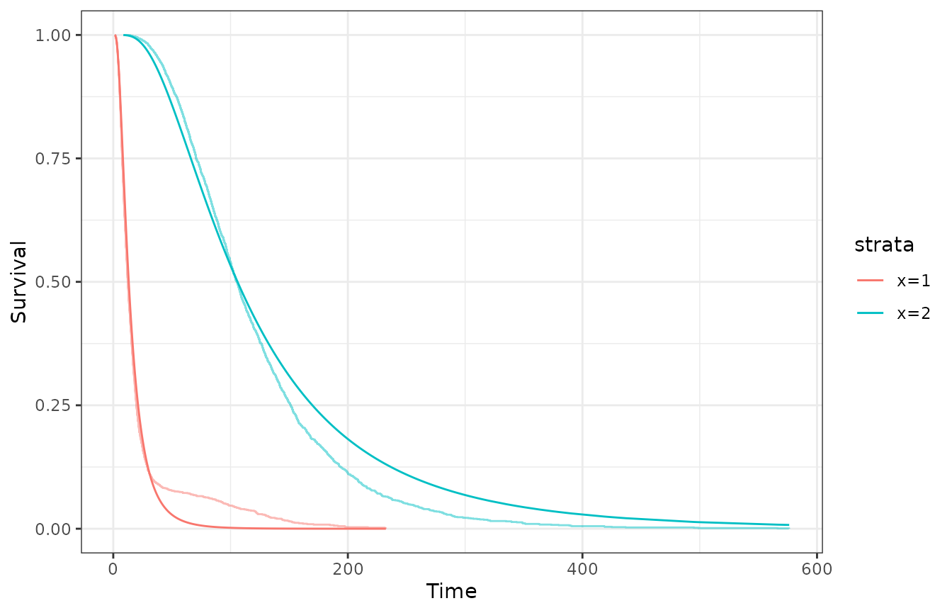
plot_fit_on_data(model_em, data = data, type = "survival")$ggplot
As expected, the fitted model isn’t that great. Increasing the
parameter number_em_search helps to find better initial
values, and thus, better fits, in exchange of computational time. We can
see how the initials values likelihood change setting the parameter
show_progress = TRUE.
model_em <- survival_ln_mixture_em(Surv(y, delta) ~ x,
  data = data,
  iter = 200,
  starting_seed = 20,
  number_em_search = 200,
  show_progress = TRUE
)
#> Initial LogLik: -30771.2
#> Previous maximum: -30771.2 | New maximum: -19065.3
#> Previous maximum: -19065.3 | New maximum: -15020.4
#> Starting EM with better initial values
#> EM Iter: 20 | 200
#> EM Iter: 40 | 200
#> EM Iter: 60 | 200
#> EM Iter: 80 | 200
#> EM Iter: 100 | 200
#> EM Iter: 120 | 200
#> EM Iter: 140 | 200
#> EM Iter: 160 | 200
#> EM Iter: 180 | 200
#> EM Iter: 200 | 200
Now, we have a maximum likelihood estimator that tries to avoid local
maximas. As before, we can use the function
plot_fit_on_data() to visualize the model’s estimated
survival on the data used to fit the model.
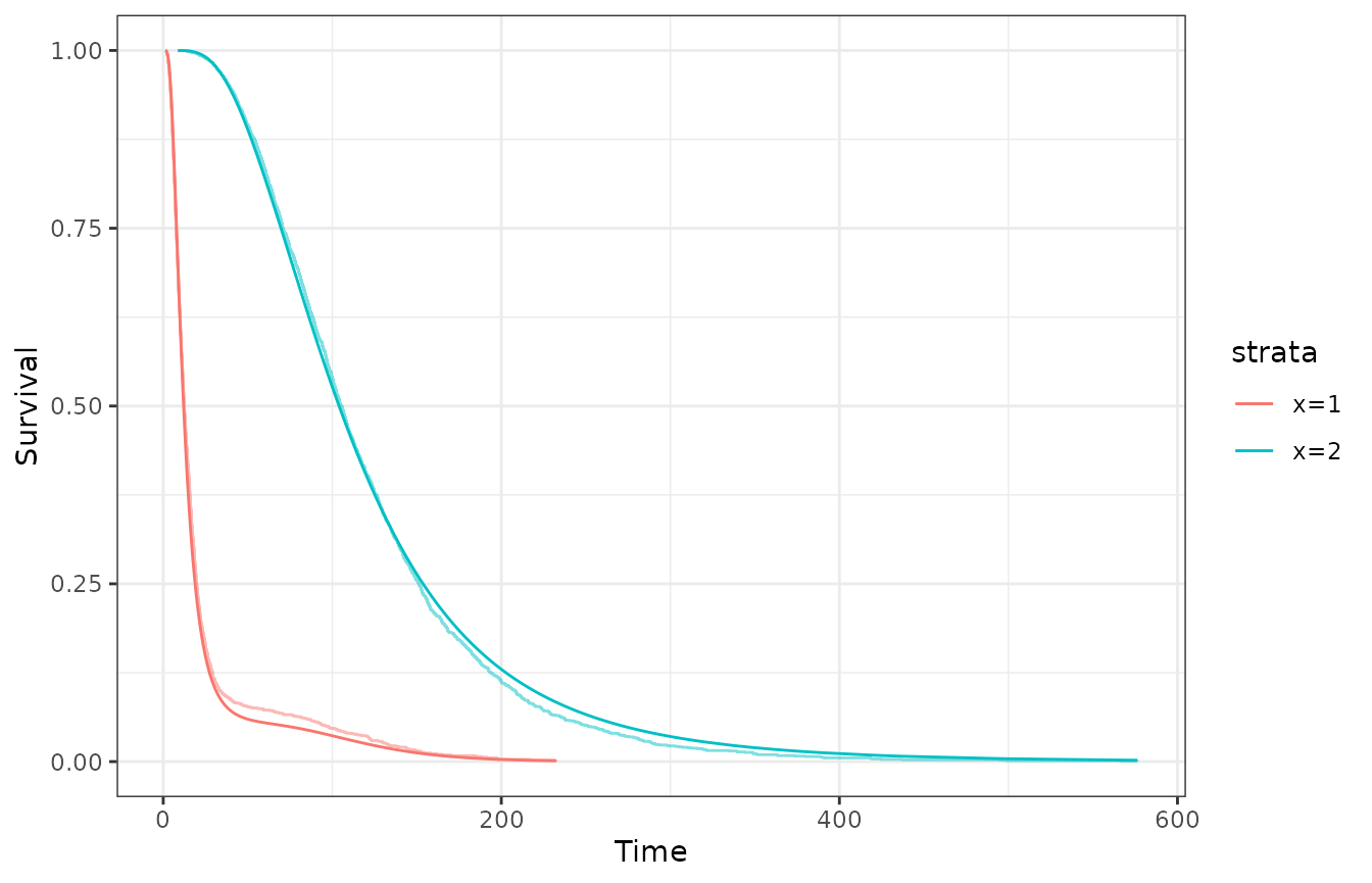
plot_fit_on_data(model_em, data = data, type = "survival")$ggplot
In fact, the model is now much better. The EM algorithm is a good alternative to the Bayesian approach when dealing with big data, but it’s important to note that it’s a maximum likelihood method, and thus, it doesn’t provide credible nor confidence intervals.