Posterior analysis with bayesplot

A survival_ln_mixture object holds the posterior chain as a ?posterior::draws_matrix object, and can be analysed using the Stan ecosystem tools, like bayesplot.

library(lnmixsurv)
library(bayesplot)
mod1 <- survival_ln_mixture(Surv(y, delta) ~ x,
  data = sim_data$data,
  starting_seed = 20, chains = 2
)

color_scheme_set("viridis")

mcmc_trace(mod1$posterior[, "eta_1"]) +
  ggplot2::theme_bw()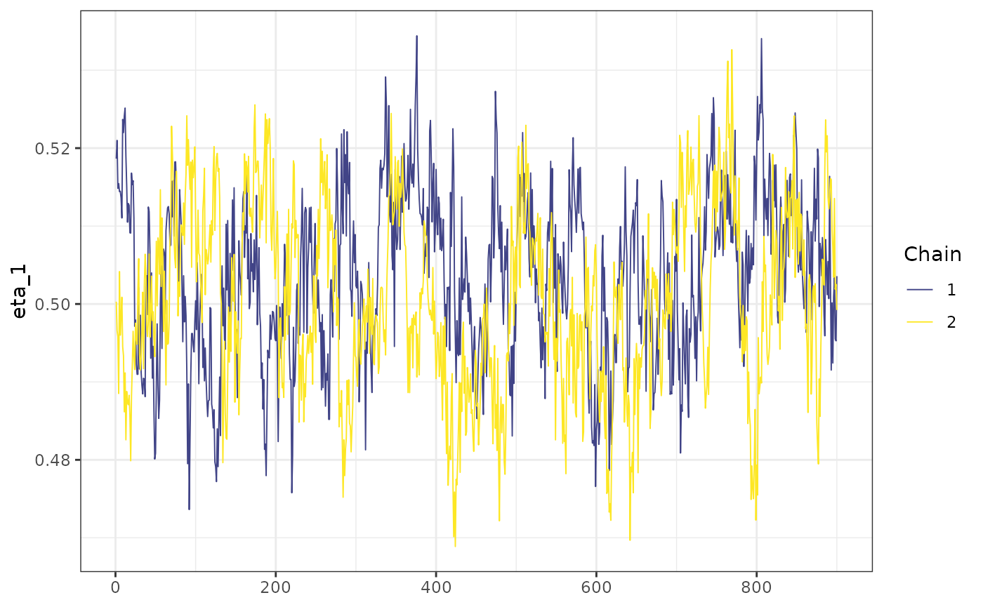

Since the seed is fixed, we expect to obtain the same chain if we run the model again, with the same seed, even if we consider the parallel option (by setting cores > 1). We can make sure this is happening by look at a small portion of the chains.

mod2 <- survival_ln_mixture(Surv(y, delta) ~ x,
  data = sim_data$data,
  starting_seed = 20, chains = 2, cores = 2
)

Here are the posterior draws for some subset of the iterations running 2 chains sequentially (mod1):

mcmc_trace(posterior::subset_draws(mod1$posterior,
  iteration = 450:600,
  variable = "eta_1"
)) +
  ggplot2::theme_bw()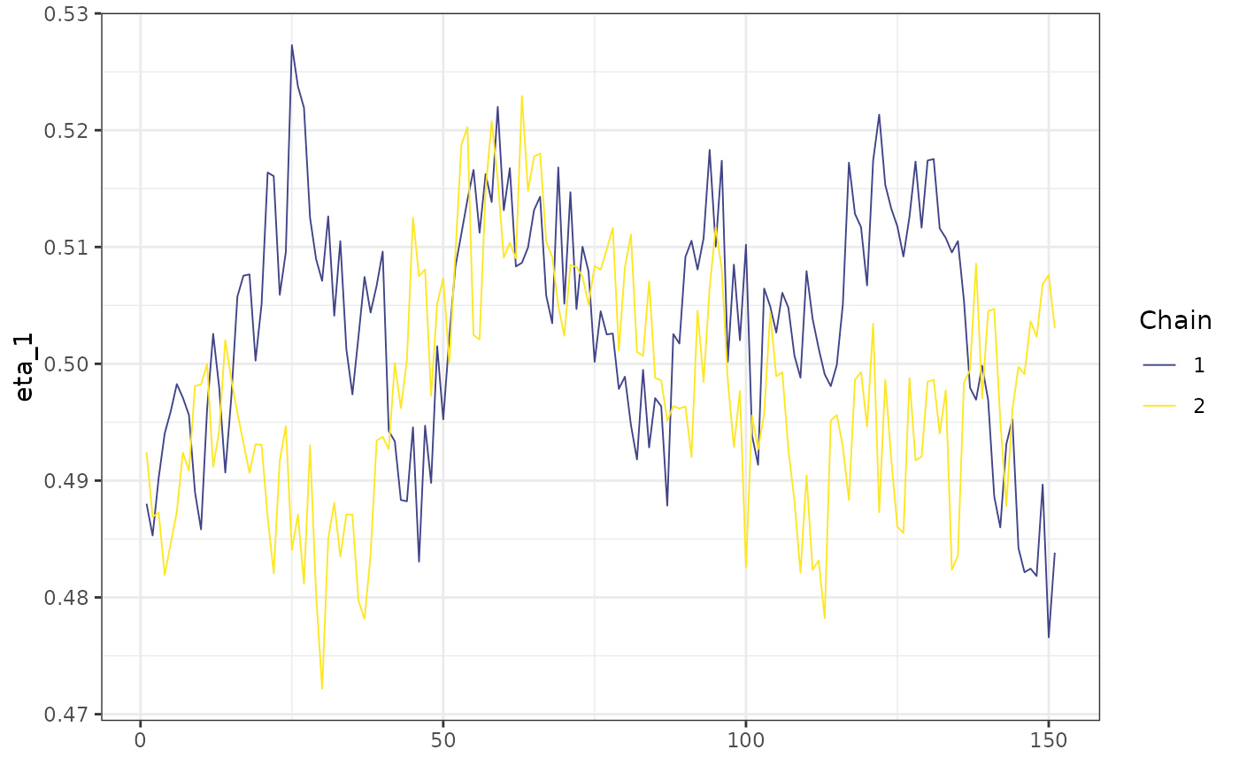

Now, the posterior draws for some subset of the iterations running 2 chains in parallel (mod2), using the same seed as mod1:

mcmc_trace(posterior::subset_draws(mod2$posterior,
  iteration = 450:600,
  variable = "eta_1"
)) +
  ggplot2::theme_bw()

As we expect, the iterations are exactly the same.